We Can Reduce the Margin of Error in an Interval Estimate of P by Doing Any of the Following Except

What Is a Confidence Interval?

A confidence interval is a blazon of interval estimate of a population parameter and is used to indicate the reliability of an guess.

Learning Objectives

Explain the principle backside confidence intervals in statistical inference

Key Takeaways

Key Points

• In inferential statistics, we use sample data to brand generalizations about an unknown population.
• A confidence interval is a type of estimate, like a sample average or sample standard deviation, only instead of being just one number it is an interval of numbers.
• The interval of numbers is an estimated range of values calculated from a given set of sample data.
• The principle behind confidence intervals was formulated to provide an reply to the question raised in statistical inference: how do we resolve the uncertainty inherent in results derived from data that are themselves merely a randomly selected subset of a population?
• Note that the confidence interval is likely to include an unknown population parameter.

Key Terms

• confidence interval: A type of interval estimate of a population parameter used to indicate the reliability of an estimate.
• population: a group of units (persons, objects, or other items) enumerated in a demography or from which a sample is fatigued
• sample: a subset of a population selected for measurement, observation, or questioning to provide statistical data about the population

Suppose you are trying to determine the boilerplate hire of a two-bedchamber flat in your town. You might look in the classified section of the newpaper, write downwardly several rents listed, and then average them together—from this you would obtain a indicate estimate of the true mean. If you are trying to determine the percentage of times you make a handbasket when shooting a basketball game, yous might count the number of shots you make, and divide that past the number of shots you attempted. In this instance, you would obtain a betoken approximate for the true proportion.

In inferential statistics, nosotros use sample information to make generalizations about an unknown population. The sample information help assist us to make an judge of a population parameter. We realize that the point estimate is virtually likely not the exact value of the population parameter, but close to it. Subsequently computing point estimates, we construct conviction intervals in which we believe the parameter lies.

A confidence interval is a blazon of estimate (like a sample boilerplate or sample standard deviation), in the class of an interval of numbers, rather than merely one number. Information technology is an observed interval (i.eastward., information technology is calculated from the observations), used to indicate the reliability of an estimate. The interval of numbers is an estimated range of values calculated from a given set of sample data. How frequently the observed interval contains the parameter is adamant by the confidence level or confidence coefficient. Note that the conviction interval is likely to include an unknown population parameter.

Philosophical Issues

The principle backside confidence intervals provides an respond to the question raised in statistical inference: how do we resolve the dubiety inherent in results derived from data that (in and of itself) is only a randomly selected subset of a population? Bayesian inference provides further answers in the form of apparent intervals.

Conviction intervals correspond to a chosen rule for determining the confidence premises; this rule is substantially determined before whatever data are obtained or before an experiment is washed. The rule is divers such that over all possible datasets that might exist obtained, at that place is a high probability ("high" is specifically quantified) that the interval determined by the rule will include the truthful value of the quantity under consideration—a fairly straightforward and reasonable way of specifying a rule for determining doubtfulness intervals.

Ostensibly, the Bayesian approach offers intervals that (bailiwick to acceptance of an interpretation of "probability" as Bayesian probability) offer the interpretation that the specific interval calculated from a given dataset has a certain probability of including the true value (conditional on the data and other information available). The conviction interval approach does not allow this, as in this formulation (and at this same stage) both the bounds of the interval and the true values are fixed values; no randomness is involved.

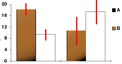
Conviction Interval: In this bar nautical chart, the tiptop ends of the bars indicate ascertainment ways and the red line segments represent the conviction intervals surrounding them. Although the confined are shown every bit symmetric in this chart, they practise non accept to be symmetric.

Interpreting a Conviction Interval

For users of frequentist methods, diverse interpretations of a confidence interval can be given.

Learning Objectives

Construct a confidence intervals based on the point estimate of the quantity being considered

Key Takeaways

Key Points

• Methods for deriving confidence intervals include descriptive statistics, likelihood theory, estimating equations, significance testing, and bootstrapping.
• The confidence interval tin can exist expressed in terms of samples: "Were this process to exist repeated on multiple samples, the calculated conviction interval would encompass the true population parameter 90% of the fourth dimension".
• The explanation of a confidence interval tin can corporeality to something like: "The conviction interval represents values for the population parameter, for which the deviation between the parameter and the observed estimate is not statistically significant at the ten% level ".
• The probability associated with a confidence interval may also be considered from a pre- experiment point of view, in the same context in which arguments for the random allocation of treatments to study items are made.

Key Terms

• frequentist: An advocate of frequency probability.
• confidence interval: A type of interval gauge of a population parameter used to indicate the reliability of an judge.

Deriving a Confidence Interval

For not-standard applications, there are several routes that might be taken to derive a rule for the structure of confidence intervals. Established rules for standard procedures might be justified or explained via several of these routes. Typically a rule for amalgam confidence intervals is closely tied to a item way of finding a indicate estimate of the quantity existence considered.

• Descriptive statistics – This is closely related to the method of moments for estimation. A simple example arises where the quantity to be estimated is the mean, in which instance a natural estimate is the sample mean. The usual arguments signal that the sample variance can exist used to gauge the variance of the sample mean. A naive conviction interval for the true hateful tin can be constructed centered on the sample mean with a width which is a multiple of the square root of the sample variance.
• Likelihood theory – The theory here is for estimates constructed using the maximum likelihood principle. Information technology provides for two means of amalgam confidence intervals (or conviction regions) for the estimates.
• Estimating equations – The estimation arroyo here can exist considered as both a generalization of the method of moments and a generalization of the maximum likelihood approach. There are corresponding generalizations of the results of maximum likelihood theory that permit conviction intervals to be constructed based on estimates derived from estimating equations.
• Significance testing – If significance tests are available for general values of a parameter, then conviction intervals/regions can be constructed past including in the [latex]100\text{p}\%[/latex] confidence region all those points for which the significance test of the naught hypothesis that the true value is the given value is non rejected at a significance level of [latex]1-\text{p}[/latex].
• Bootstrapping – In situations where the distributional assumptions for the above methods are uncertain or violated, resampling methods allow construction of confidence intervals or prediction intervals. The observed data distribution and the internal correlations are used as the surrogate for the correlations in the wider population.

Meaning and Estimation

For users of frequentist methods, various interpretations of a conviction interval tin can be given:

• The conviction interval tin be expressed in terms of samples (or repeated samples): "Were this procedure to be repeated on multiple samples, the calculated confidence interval (which would differ for each sample) would cover the true population parameter 90% of the fourth dimension. " Notation that this does not refer to repeated measurement of the same sample, merely repeated sampling.
• The explanation of a confidence interval can amount to something like: "The confidence interval represents values for the population parameter, for which the difference between the parameter and the observed judge is not statistically significant at the 10% level. " In fact, this relates to one particular way in which a confidence interval may be constructed.
• The probability associated with a confidence interval may also be considered from a pre-experiment indicate of view, in the same context in which arguments for the random resource allotment of treatments to written report items are made. Here, the experimenter sets out the way in which they intend to calculate a confidence interval. Before performing the actual experiment, they know that the stop calculation of that interval will accept a certain take chances of covering the true but unknown value. This is very similar to the "repeated sample" interpretation in a higher place, except that it avoids relying on considering hypothetical repeats of a sampling procedure that may not be repeatable in any meaningful sense.

In each of the to a higher place, the following applies: If the true value of the parameter lies outside the 90% conviction interval once information technology has been calculated, then an upshot has occurred which had a probability of 10% (or less) of happening by take chances.

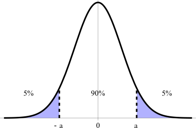
Confidence Interval: This effigy illustrates a ninety% conviction interval on a standard normal curve.

Caveat Emptor and the Gallup Poll

Readers of polls, such every bit the Gallup Poll, should do Caveat Emptor by taking into account the poll's margin of error.

Learning Objectives

Explain how margin of error plays a significant role in making purchasing decisions

Central Takeaways

Key Points

• Historically, the Gallup Poll has measured and tracked the public's attitudes apropos most every political, social, and economic effect of the 24-hour interval, including highly sensitive or controversial subjects.
• Caveat emptor is Latin for "let the heir-apparent beware"—the belongings law principle that controls the auction of real holding afterwards the date of endmost, but may also apply to sales of other appurtenances.
• The margin of fault is usually divers as the "radius" (or one-half the width) of a confidence interval for a detail statistic from a survey.
• The larger the margin of mistake, the less confidence one should take that the poll's reported results are shut to the "true" figures — that is, the figures for the whole population.
• Like confidence intervals, the margin of error tin be defined for whatsoever desired confidence level, merely normally a level of xc%, 95% or 99% is called (typically 95%).

Fundamental Terms

• caveat emptor: Latin for "allow the buyer beware"—the belongings law principle that controls the sale of existent property after the date of closing, simply may besides apply to sales of other goods.
• margin of fault: An expression of the lack of precision in the results obtained from a sample.

Gallup Poll

The Gallup Poll is the partitioning of the Gallup Company that regularly conducts public opinion polls in more than than 140 countries around the earth. Gallup Polls are often referenced in the mass media as a reliable and objective measurement of public opinion. Gallup Poll results, analyses, and videos are published daily on Gallup.com in the class of data-driven news.

Since inception, Gallup Polls have been used to measure and track public attitudes concerning a broad range of political, social, and economic issues (including highly sensitive or controversial subjects). Full general and regional-specific questions, developed in collaboration with the globe's leading behavioral economists, are organized into powerful indexes and topic areas that correlate with existent-globe outcomes.

Caveat Emptor

Caveat emptor is Latin for "permit the buyer beware." By and large, caveat emptor is the property constabulary principle that controls the sale of real property after the appointment of endmost, but may also utilize to sales of other appurtenances. Under its principle, a buyer cannot recover damages from a seller for defects on the property that render the belongings unfit for ordinary purposes. The only exception is if the seller actively conceals latent defects, or otherwise states material misrepresentations amounting to fraud.

This principle can also be applied to the reading of polling data. The reader should "beware" of possible errors and biases present that might skew the information beingness represented. Readers should pay close attention to a poll's margin of mistake.

Margin of Error

The margin of error statistic expresses the amount of random sampling error in a survey'southward results. The larger the margin of error, the less conviction one should have that the poll'due south reported results represent "true" figures (i.east., figures for the whole population). Margin of fault occurs whenever a population is incompletely sampled.

The margin of fault is usually divers equally the "radius" (half the width) of a confidence interval for a particular statistic from a survey. When a single, global margin of mistake is reported, it refers to the maximum margin of error for all reported percentages using the full sample from the survey. If the statistic is a percentage, this maximum margin of error is calculated as the radius of the confidence interval for a reported per centum of fifty%.

For example, if the true value is fifty percent points, and the statistic has a confidence interval radius of 5 percentage points, and then we say the margin of error is 5 percentage points. Equally another example, if the truthful value is 50 people, and the statistic has a confidence interval radius of v people, then nosotros might say the margin of error is 5 people.

In some cases, the margin of error is not expressed as an "absolute" quantity; rather, it is expressed as a "relative" quantity. For example, suppose the true value is l people, and the statistic has a confidence interval radius of 5 people. If we apply the "absolute" definition, the margin of error would exist v people. If we use the "relative" definition, then nosotros express this absolute margin of error as a pct of the true value. So in this example, the accented margin of fault is 5 people, but the "percent relative" margin of error is x% (10% of 50 people is 5 people).

Similar conviction intervals, the margin of error tin be divers for any desired conviction level, but usually a level of 90%, 95% or 99% is chosen (typically 95%). This level is the probability that a margin of error around the reported percentage would include the "true" percentage. Along with the conviction level, the sample design for a survey (in particular its sample size) determines the magnitude of the margin of fault. A larger sample size produces a smaller margin of error, all else remaining equal.

If the exact confidence intervals are used, then the margin of fault takes into account both sampling mistake and not-sampling error. If an approximate confidence interval is used (for example, by assuming the distribution is normal and and then modeling the confidence interval accordingly), then the margin of mistake may only have random sampling error into account. It does non correspond other potential sources of error or bias, such equally a non-representative sample-design, poorly phrased questions, people lying or refusing to answer, the exclusion of people who could non be contacted, or miscounts and miscalculations.

Different Confidence Levels

For a simple random sample from a large population, the maximum margin of mistake is a elementary re-expression of the sample size [latex]\text{n}[/latex]. The numerators of these equations are rounded to two decimal places.

• Margin of error at 99% conviction [latex]\displaystyle \approx \frac { ane.29 }{ \sqrt { \text{northward} } }[/latex]
• Margin of mistake at 95% confidence [latex]\displaystyle \approx \frac { 0.98 }{ \sqrt { \text{n} } }[/latex]
• Margin of error at xc% confidence [latex]\displaystyle \approx \frac { 0.82 }{ \sqrt { \text{due north} } }[/latex]

If an article almost a poll does non report the margin of error, but does state that a simple random sample of a certain size was used, the margin of error can be calculated for a desired degree of confidence using one of the in a higher place formulae. Also, if the 95% margin of error is given, one can find the 99% margin of mistake by increasing the reported margin of error by about 30%.

As an example of the in a higher place, a random sample of size 400 volition give a margin of error, at a 95% confidence level, of [latex]\frac{0.98}{20}[/latex] or 0.049 (but under 5%). A random sample of size one,600 volition give a margin of mistake of [latex]\frac{0.98}{twoscore}[/latex], or 0.0245 (just under 2.five%). A random sample of size 10,000 will give a margin of fault at the 95% confidence level of [latex]\frac{0.98}{100}[/latex], or 0.0098 – simply nether 1%.

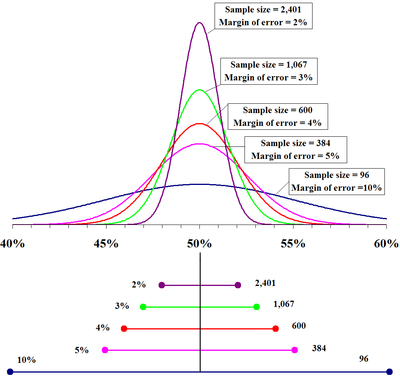
Margin for Error: The top portion of this graphic depicts probability densities that show the relative likelihood that the "truthful" percentage is in a particular surface area given a reported pct of 50%. The bottom portion shows the 95% confidence intervals (horizontal line segments), the respective margins of mistake (on the left), and sample sizes (on the right). In other words, for each sample size, 1 is 95% confident that the "truthful" percent is in the region indicated by the corresponding segment. The larger the sample is, the smaller the margin of error is.

Level of Conviction

The proportion of confidence intervals that contain the true value of a parameter will match the confidence level.

Learning Objectives

Explicate the use of confidence intervals in estimating population parameters

Key Takeaways

Key Points

• The presence of a confidence level is guaranteed past the reasoning underlying the construction of confidence intervals.
• Confidence level is represented by a percentage.
• The desired level of confidence is fix by the researcher (not adamant by data ).
• In applied practise, conviction intervals are typically stated at the 95% confidence level.

Fundamental Terms

• confidence level: The probability that a measured quantity will fall within a given conviction interval.

If confidence intervals are constructed across many separate data analyses of repeated (and peradventure different) experiments, the proportion of such intervals that contain the true value of the parameter volition match the conviction level. This is guaranteed past the reasoning underlying the construction of confidence intervals.

Confidence intervals consist of a range of values (interval) that act equally adept estimates of the unknown population parameter. Notwithstanding, in infrequent cases, none of these values may comprehend the value of the parameter. The level of confidence of the conviction interval would bespeak the probability that the confidence range captures this true population parameter given a distribution of samples. It does not draw whatsoever unmarried sample. This value is represented past a per centum, so when we say, "we are 99% confident that the true value of the parameter is in our confidence interval," we express that 99% of the observed confidence intervals will hold the true value of the parameter.

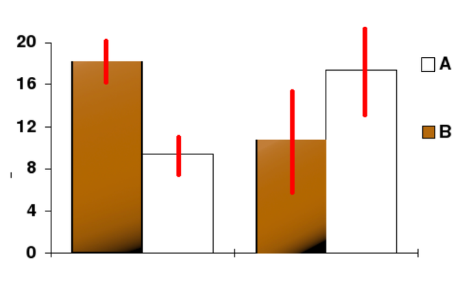
Confidence Level: In this bar chart, the top ends of the confined indicate ascertainment ways and the red line segments correspond the confidence intervals surrounding them. Although the confined are shown equally symmetric in this chart, they practice not accept to be symmetric.

Later a sample is taken, the population parameter is either in the interval made or non — there is no chance. The desired level of confidence is set by the researcher (not adamant by information). If a corresponding hypothesis exam is performed, the conviction level is the complement of respective level of significance (i.due east., a 95% conviction interval reflects a significance level of 0.05).

In applied exercise, conviction intervals are typically stated at the 95% confidence level. However, when presented graphically, confidence intervals can be shown at several confidence levels (for instance, 50%, 95% and 99%).

Determining Sample Size

A major factor determining the length of a conviction interval is the size of the sample used in the estimation procedure.

Learning Objectives

Assess the near advisable way to choose a sample size in a given situation

Fundamental Takeaways

Cardinal Points

• Sample size determination is the human action of choosing the number of observations or replicates to include in a statistical sample.
• The sample size is an of import characteristic of any empirical study in which the goal is to make inferences most a population from a sample.
• In practice, the sample size used in a study is determined based on the expense of information collection and the need to take sufficient statistical power.
• Larger sample sizes generally atomic number 82 to increased precision when estimating unknown parameters.

Central Terms

• law of large numbers: The statistical trend toward a fixed ratio in the results when an experiment is repeated a big number of times.
• primal limit theorem: The theorem that states: If the sum of contained identically distributed random variables has a finite variance, then information technology will exist (approximately) unremarkably distributed.
• Stratified Sampling: A method of sampling that involves dividing members of the population into homogeneous subgroups before sampling.

Sample size, such as the number of people taking part in a survey, determines the length of the estimated conviction interval. Sample size decision is the act of choosing the number of observations or replicates to include in a statistical sample. The sample size is an important characteristic of any empirical study in which the goal is to make inferences most a population from a sample.

In practice, the sample size used in a written report is adamant based on the expense of data collection and the need to have sufficient statistical power. In complicated studies at that place may exist several different sample sizes involved. For example, in a survey sampling involving stratified sampling there would be dissimilar sample sizes for each population. In a census, information are collected on the unabridged population, hence the sample size is equal to the population size. In experimental blueprint, where a study may be divided into different treatment groups, there may exist different sample sizes for each group.

Sample sizes may exist called in several different means:

• expedience, including those items readily available or convenient to collect (choice of minor sample sizes, though sometimes necessary, can issue in wide confidence intervals or risks of errors in statistical hypothesis testing)
• using a target variance for an estimate to be derived from the sample eventually obtained
• using a target for the power of a statistical test to be practical one time the sample is collected

Larger sample sizes by and large lead to increased precision when estimating unknown parameters. For example, if we wish to know the proportion of a certain species of fish that is infected with a pathogen, we would by and large have a more authentic gauge of this proportion if we sampled and examined 200, rather than 100 fish. Several central facts of mathematical statistics describe this phenomenon, including the constabulary of large numbers and the central limit theorem.

In some situations, the increase in accuracy for larger sample sizes is minimal, or even non-real. This tin can result from the presence of systematic errors or potent dependence in the data, or if the data follow a heavy-tailed distribution.

Sample sizes are judged based on the quality of the resulting estimates. For case, if a proportion is being estimated, one may wish to have the 95% confidence interval be less than 0.06 units wide. Alternatively, sample size may be assessed based on the power of a hypothesis test. For case, if we are comparing the support for a certain political candidate among women with the support for that candidate among men, we may wish to have 80% ability to detect a deviation in the support levels of 0.04 units.

Calculating the Sample Size [latex]\text{north}[/latex]

If researchers desire a specific margin of error, then they can utilise the error leap formula to summate the required sample size. The fault bound formula for a population proportion is:

[latex]\displaystyle \text{EBP} = \text{z}_{\frac{\alpha}{2}}\sqrt{\frac{\text{p}'\text{q}'}{\text{due north}}}[/latex]

Solving for [latex]\text{n}[/latex] gives an equation for the sample size:

[latex]\text{northward}=\frac{\left(\text{z}_{\frac{\alpha}{2}}\right)^2\text{p}'\text{q}'}{\text{EBP}^two}[/latex]

Confidence Interval for a Population Proportion

The procedure to notice the conviction interval and the confidence level for a proportion is similar to that for the population hateful.

Learning Objectives

Calculate the confidence interval given the estimated proportion of successes

Key Takeaways

Cardinal Points

• Confidence intervals can exist calculated for the truthful proportion of stocks that get up or down each week and for the true proportion of households in the United States that ain personal computers.
• To grade a proportion, take [latex]\text{X}[/latex] (the random variable for the number of successes) and divide information technology by [latex]\text{n}[/latex] (the number of trials, or the sample size).
• If we split up the random variable by [latex]\text{north}[/latex], the hateful by [latex]\text{n}[/latex], and the standard deviation past [latex]\text{n}[/latex], we go a normal distribution of proportions with [latex]\text{P}'[/latex], chosen the estimated proportion, as the random variable.
• This formula is similar to the error spring formula for a mean, except that the "appropriate standard deviation" is different.

Key Terms

• error jump: The margin or error that depends on the conviction level, sample size, and the estimated (from the sample) proportion of successes.

During an ballot year, we oftentimes read news articles that state confidence intervals in terms of proportions or percentages. For instance, a poll for a item presidential candidate might show that the candidate has forty% of the vote, within 3 pct points. Often, election polls are calculated with 95% confidence. This mean that pollsters are 95% confident that the true proportion of voters who favor the candidate lies between 0.37 and 0.43:

[latex](0.twoscore-0.03, 0.forty+0.03)[/latex]

Investors in the stock market are interested in the true proportion of stock values that go upwards and down each week. Businesses that sell personal computers are interested in the proportion of households (say, in the United States) that own personal computers. Conviction intervals can exist calculated for both scenarios.

Although the process to detect the confidence interval, sample size, error bound, and confidence level for a proportion is similar to that for the population hateful, the formulas are dissimilar.

Proportion Problems

How do y'all know if you are dealing with a proportion problem? Showtime, the underlying distribution is binomial (i.e., there is no mention of a mean or boilerplate). If [latex]\text{X}[/latex] is a binomial random variable, so [latex]\text{X}\sim \text{B}(\text{northward},\text{p})[/latex] where [latex]\text{n}[/latex] is the number of trials and [latex]\text{p}[/latex] is the probability of a success. To form a proportion, take [latex]\text{X}[/latex] (the random variable for the number of successes) and split information technology by [latex]\text{due north}[/latex] (the number of trials or the sample size). The random variable [latex]\text{P}'[/latex] (read "[latex]\text{P}[/latex] prime") is that proportion:

[latex]\displaystyle { \text{P}}'=\frac { \text{X} }{ \text{northward} }[/latex]

Sometimes the random variable is denoted equally [latex]\hat{\text{P}}[/latex] (read equally [latex]\text{P}[/latex] hat)

When [latex]\text{n}[/latex] is large and [latex]\text{p}[/latex] is not close to 0 or 1, nosotros can employ the normal distribution to approximate the binomial.

[latex]\text{X}\sim \text{N}\left( \text{n}\cdot \text{p},\sqrt { \text{n}\cdot \text{p}\cdot \text{q} } \right)[/latex]

If we divide the random variable by [latex]\text{due north}[/latex], the mean past [latex]\text{n}[/latex], and the standard deviation by [latex]\text{due north}[/latex], we get a normal distribution of proportions with [latex]\text{P}'[/latex], called the estimated proportion, as the random variable. (Recall that a proportion is the number of successes divided by [latex]\text{n}[/latex].)

[latex]\displaystyle \frac { \text{X} }{ \text{north} } ={ \text{P}}'\sim \text{North}\left( \frac { \text{n}-\text{p} }{ \text{northward} },\frac { \sqrt { \text{n}\cdot \text{p}\cdot \text{q} } }{ \text{due north} } \right)[/latex]

Using algebra to simplify:

[latex]\displaystyle \frac { \sqrt { \text{n}\cdot \text{p}\cdot \text{q} } }{ \text{n} } =\sqrt { \frac { \text{p}\cdot \text{q} }{ \text{northward} } }[/latex]

[latex]\text{P}'[/latex] follows a normal distribution for proportions:

[latex]{ \text{P}}'\sim \text{N}\left( \text{p},\sqrt { \frac { \text{p}\cdot \text{q} }{ \text{north} } } \right)[/latex]

The confidence interval has the form [latex](\text{p}'-\text{EBP}, \text{p}'+\text{EBP})[/latex].

• [latex]\displaystyle{{ \text{p} }'=\frac { \text{x} }{ \text{n} }}[/latex]
• [latex]\text{p}'[/latex] is the estimated proportion of successes ([latex]\text{p}'[/latex] is a indicate judge for [latex]\text{p}[/latex], the true proportion)
• [latex]\text{10}[/latex] is the number of successes
• [latex]\text{n}[/latex] is the size of the sample

The error bound for a proportion is seen in the formula in:

[latex]\displaystyle \text{EBP} = \text{z}_{\frac{\alpha}{2}}\sqrt{\frac{\text{p}'\text{q}'}{\text{n}}}[/latex]

where [latex]\text{q}'=1-\text{p}'[/latex].

This formula is like to the error bound formula for a mean, except that the "appropriate standard difference" is dissimilar. For a mean, when the population standard deviation is known, the appropriate standard deviation that we utilise is [latex]\frac { \sigma }{ \sqrt { \text{northward} } }[/latex]. For a proportion, the appropriate standard deviation is [latex]\sqrt { \frac { \text{p}\cdot \text{q} }{ \text{n} } }[/latex].

Nonetheless, in the error bound formula, we utilise [latex]\sqrt { \frac { { \text{p} }^{ ' }\cdot { \text{q} }^{ ' } }{ \text{northward} } }[/latex] as the standard deviation, instead of [latex]\sqrt { \frac { \text{p}\cdot \text{q} }{ \text{northward} } }[/latex].

In the error bound formula, the sample proportions [latex]\text{p}'[/latex] and [latex]\text{q}'[/latex] are estimates of the unknown population proportions [latex]\text{p}[/latex] and [latex]\text{q}[/latex]. The estimated proportions [latex]\text{p}'[/latex] and [latex]\text{q}'[/latex] are used considering [latex]\text{p}[/latex] and [latex]\text{q}[/latex] are not known. [latex]\text{p}'[/latex] and [latex]\text{q}'[/latex] are calculated from the information. [latex]\text{p}'[/latex] is the estimated proportion of successes. [latex]\text{q}'[/latex] is the estimated proportion of failures.

The confidence interval tin can but exist used if the number of successes [latex]\text{np}'[/latex] and the number of failures [latex]\text{nq}'[/latex] are both larger than v.

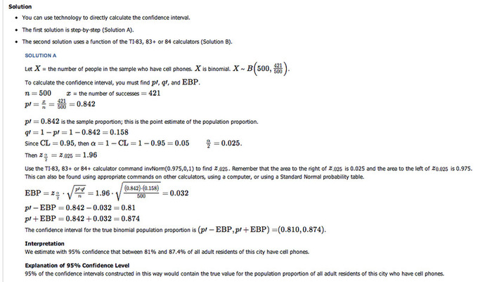
Solution: This image shows the solution to our example.

Confidence Interval for a Population Mean, Standard Divergence Known

In this department, we outline an example of finding the confidence interval for a population mean when we know the standard deviation.

Learning Objectives

Calculate the conviction interval for a mean given that standard departure is known

Central Takeaways

Fundamental Points

• Our example is for scores on exams in statistics that are ordinarily distributed with an unknown population mean and a population standard deviation of 3 points.
• A random sample of 36 scores is taken and gives a sample hateful (sample mean score) of 68.
• The xc% confidence interval for the hateful score is [latex](67.1775, 68.8225)[/latex].
• We are 90% confident that the interval from 67.1775% to 68.8225% contains the true mean score of all the statistics exams: 90% of all confidence intervals constructed in this way contain the truthful mean statistics exam score.

Key Terms

• margin of error: An expression of the lack of precision in the results obtained from a sample.
• conviction interval: A type of interval judge of a population parameter used to bespeak the reliability of an gauge.

Step Past Step Example of a Confidence Interval for a Mean—Standard Deviation Known

Suppose scores on exams in statistics are normally distributed with an unknown population mean, and a population standard deviation of iii points. A random sample of 36 scores is taken and gives a sample mean (sample mean score) of 68. To find a 90% confidence interval for the true (population) mean of statistics exam scores, we accept the following guidelines:

1. Programme: Land what we need to know.
2. Model: Remember virtually the assumptions and cheque the conditions.
3. Land the parameters and the sampling model.
4. Mechanics: [latex]\text{CL} = 0.90[/latex], so [latex]\alpha = 1-\text{CL} = ane-0.90 = 0.ten[/latex]; [latex]\alpha_{0.05}[/latex] is [latex]i-0.05 = 0.95[/latex]; So [latex]\text{z}_{0.05} = i.645[/latex]
5. Conclusion: Interpret your result in the proper context, and relate information technology to the original question.

1. In our example, we are asked to find a ninety% confidence interval for the mean examination score, [latex]\mu[/latex], of statistics students.

Nosotros accept a sample of 68 students.

ii. We know the population standard deviation is 3. We take the following conditions:

• Randomization Condition: The sample is a random sample.
• Independence Supposition: Information technology is reasonable to call back that the exam scores of 36 randomly selected students are independent.
• 10% Condition: We assume the statistic student population is over 360 students, so 36 students is less than ten% of the population.
• Sample Size Condition: Since the distribution of the stress levels is normal, our sample of 36 students is big enough.

3. The conditions are satisfied and [latex]\sigma[/latex] is known, so nosotros volition use a confidence interval for a mean with known standard divergence. Nosotros need the sample mean and margin of error (ME):

[latex]\bar { \text{x} } =68 \\ \sigma =3 \\ \text{north}=36 \\ \text{ME}={ \text{z} }_{ \frac { \alpha }{ 2 } }\left( \dfrac { \sigma }{ \sqrt { \text{northward} } } \right)[/latex]

4. below shows the steps for calculating the conviction interval.

[latex]\displaystyle {\text{ME} = 1.645\cdot \frac{3}{\sqrt{36}} = 0.8225 \\ \bar{x} - \text{ME} = 68-0.8225 = 67.1775 \\ \bar{x} + \text{ME} = 68+0.8225 = 68.8225}[/latex]

The 90% conviction interval for the mean score is [latex](67.1775, 68.8225)[/latex].

Graphical Representation: This figure is a graphical representation of the conviction interval we calculated in this instance.

v. In decision, we are 90% confident that the interval from 67.1775 to 68.8225 contains the true mean score of all the statistics exams. ninety% of all confidence intervals constructed in this fashion contain the truthful hateful statistics test score.

Confidence Interval for a Population Mean, Standard Deviation Not Known

In this section, we outline an example of finding the confidence interval for a population mean when we do not know the standard departure.

Learning Objectives

Calculate the confidence interval for the hateful when the standard deviation is unknown

Key Takeaways

Key Points

• Our case is for a written report of acupuncture to make up one's mind how effective it is in relieving pain.
• We measure sensory rates for 15 random subjects, with the results being:8.half-dozen, ix.4, 7.9, 6.viii, 8.3, 7.3, 9.2, 9.6, 8.7, xi.iv, x.3, 5.four, 8.1, 5.5, 6.ix.
• Nosotros want to use the sample data to construct a 95% confidence interval for the hateful sensory charge per unit for the populations (assumed normal) from which we took this data.
• The 95% confidence interval for the mean score is [latex](7.30, ix.15)[/latex].
• We are 95% confident that the interval from 7.30 to 9.15 contains the true mean score of all the sensory rates—95% of all confidence intervals synthetic in this way contain the truthful mean sensory rate score.

Key Terms

• margin of error: An expression of the lack of precision in the results obtained from a sample.
• conviction interval: A type of interval estimate of a population parameter used to indicate the reliability of an guess.

Pace By Step Instance of a Confidence Interval for a Mean—Standard Divergence Unknown

Suppose you lot exercise a report of acupuncture to decide how effective it is in relieving hurting. You measure sensory rates for xv random subjects with the results given beneath:

8.6, 9.4, 7.9, 6.8, 8.3, seven.three, 9.2, 9.6, viii.7, 11.4, 10.3, 5.iv, viii.1, 5.5, half-dozen.nine.

Utilize the sample data to construct a 95% confidence interval for the mean sensory rate for the populations (causeless normal) from which yous took this data.

We take the following guidelines for such a trouble:

1. Plan: State what nosotros demand to know.
2. Model: Think about the assumptions and check the conditions.
3. Land the parameters and the sampling model.
4. Mechanics: [latex]\text{CL} = 0.95[/latex], so [latex]\alpha = i-\text{CL} = 1-0.95 = 0.05[/latex]. The area to the right of [latex]\text{t}_{0.25}[/latex] is [latex]i-0.025 = 0.975[/latex]; then [latex]\text{t}_{0.025, fourteen} = 2.14[/latex].
5. Determination: Interpret your result in the proper context, and relate it to the original question.

i. In our instance, we are asked to find a 95% confidence interval for the mean sensory rate, [latex]\mu[/latex], of acupuncture subjects. We have a sample of 15 rates. We exercise not know the population standard deviation.

2. Nosotros have the following conditions:

• Randomization Status: The sample is a random sample.
• Independence Assumption: Information technology is reasonable to think that the sensory rates of 15 subjects are independent.
• x% Condition: We assume the acupuncture population is over 150, so 15 subjects is less than 10% of the population.
• Sample Size Condition: Since the distribution of mean sensory rates is normal, our sample of 15 is large plenty.
• Nearly Normal Status: We should do a box plot and histogram to bank check this. Even though the data is slightly skewed, it is unimodal (and there are no outliers) so we can use the model.

3. The weather condition are satisfied and [latex]\sigma[/latex] is unknown, so we will use a confidence interval for a mean with unknown standard deviation. We demand the sample mean and margin of fault (ME).

[latex]\overline { \text{x} } =8.2267;\text{ southward}=1.6722;\text{ n}=fifteen;[/latex]

[latex]\text{df}=15-1=14;\text{ME}={ \text{t} }_{ \frac { \text{a} }{ 2 } }\left( \frac { 8 }{ \sqrt { \text{n} } } \right)[/latex]

4. [latex]\text{ME} = 2.fourteen[/latex]

[latex]\left( \frac { one.6722 }{ \sqrt { 15 } } \right) =0.924[/latex]

[latex]\overline { \text{x} } =\text{ME}=8.2267-0.9240=7.3027[/latex]

[latex]\overline { \text{ten} } =\text{ME}=8.2267+0.9240=9.1507[/latex]

The 95% conviction interval for the mean score is [latex](seven.30, 9.fifteen)[/latex].

Graphical Representation: This effigy is a graphical representation of the conviction interval nosotros calculated in this case.

5. Nosotros are 95% confident that the interval from seven.30 to 9.fifteen contains the true hateful score of all the sensory rates. 95% of all conviction intervals constructed in this way contain the truthful mean sensory rate score.

Box Plot: This effigy is a box plot for the information fix in our instance.

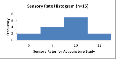
Histogram: This figure is a histogram for the data set in our example.

Estimating a Population Variance

The chi-square distribution is used to construct confidence intervals for a population variance.

Learning Objectives

Construct a confidence interval in a chi-square distribution

Key Takeaways

Key Points

• The chi-square distribution with [latex]\text{k}[/latex] degrees of freedom is the distribution of a sum of the squares of [latex]\text{thou}[/latex] contained standard normal random variables.
• The chi-square distribution enters all analyses of variance problems via its office in the [latex]\text{F}[/latex]-distribution, which is the distribution of the ratio of 2 independent chi-squared random variables, each divided by their respective degrees of liberty.
• To course a conviction interval for the population variance, use the chi-square distribution with degrees of freedom equal to one less than the sample size: [latex]\text{d.f.} = \text{n}-1[/latex].

Key Terms

• chi-square distribution: With [latex]\text{k}[/latex] degrees of liberty, the distribution of a sum of the squares of [latex]\text{one thousand}[/latex] contained standard normal random variables.
• degree of freedom: Whatever unrestricted variable in a frequency distribution.

In many manufacturing processes, information technology is necessary to control the amount that the procedure varies. For example, an automobile part manufacturer must produce thousands of parts that can be used in the manufacturing process. It is imperative that the parts vary picayune or not at all. How might the manufacturer measure and, consequently, control the amount of variation in the automobile parts? A chi-foursquare distribution can be used to construct a conviction interval for this variance.

The chi-square distribution with a [latex]\text{k}[/latex] degree of freedom is the distribution of a sum of the squares of [latex]\text{k}[/latex] independent standard normal random variables. It is i of the most widely used probability distributions in inferential statistics (e.g., in hypothesis testing or in construction of confidence intervals). The chi-squared distribution is a special case of the gamma distribution and is used in the common chi-squared tests for goodness of fit of an observed distribution to a theoretical one, the independence of ii criteria of classification of qualitative data, and in confidence interval estimation for a population standard deviation of a normal distribution from a sample standard deviation. In fact, the chi-square distribution enters all analyses of variance problems via its office in the [latex]\text{F}[/latex]-distribution, which is the distribution of the ratio of ii independent chi-squared random variables, each divided past their respective degrees of liberty.

The chi-square distribution is a family of curves, each determined past the degrees of freedom. To form a confidence interval for the population variance, utilize the chi-square distribution with degrees of liberty equal to one less than the sample size:

[latex]\text{d.f.} = \text{northward}-1[/latex]

There are ii critical values for each level of confidence:

1. The value of [latex]{ \text{X} }_{ \text{R} }^{ 2 }[/latex]represents the correct-tail critical value.
2. The value of [latex]{ \text{Ten} }_{ \text{50} }^{ two }[/latex]represents the left-tail disquisitional value.

Amalgam a Confidence Interval

As example, imagine you randomly select and weigh 30 samples of an allergy medication. The sample standard deviation is 1.two milligrams. Assuming the weights are normally distributed, construct 99% confidence intervals for the population variance and standard deviation.

The areas to the left and right of [latex]{ \text{X} }_{ \text{R} }^{ 2 }[/latex]and left of [latex]{ \text{X} }_{ \text{Fifty} }^{ 2 }[/latex] are:

Expanse to the correct of [latex]{ \text{Ten} }_{ \text{R} }^{ 2 } = \frac{i-0.99}{2} = 0.005[/latex]

Expanse to the left of [latex]{ \text{X} }_{ \text{L} }^{ two } = \frac{1+0.99}{2} = 0.995[/latex]

Using the values [latex]\text{n}=xxx[/latex], [latex]\text{d.f.} = 29[/latex] and [latex]\text{c}=0.99[/latex], the disquisitional values are 52.336 and 13.121, respectively. Note that these critical values are institute on the chi-square critical value table, similar to the tabular array used to notice [latex]\text{z}[/latex]-scores.

Using these disquisitional values and [latex]\text{southward}=ane.2[/latex], the confidence interval for [latex]\text{due south}^two[/latex] is as follows:

Right endpoint:

[latex]\displaystyle \frac{(\text{north}-i)\text{s}^2}{\chi_\text{L}^ii} = \frac{(30-one)(1.two)^2}{xiii.121} \approx iii.183[/latex]

Left endpoint:

[latex]\displaystyle \frac{(\text{n}-1)\text{s}^2}{\chi_\text{R}^2} = \frac{(30-1)(1.2)^2}{52.336} \approx 0.798[/latex]

So, with 99% confidence, we can say that the population variance is between 0.798 and iii.183.

houstonfusent.blogspot.com

Source: https://courses.lumenlearning.com/boundless-statistics/chapter/confidence-intervals/

Share this post